
ABSTRACT
Bayesian statistics assesses probabilistically all sources of uncertainty involved in a statistical study and uses Bayes’ theorem to sequentially update the information generated in the different phases of the study. The characteristics of Bayesian inference make it particularly useful for the treatment of cardiological data from experimental or observational studies including different sources of variability, and complexity. This paper presents the basic concepts of Bayesian statistics associated with the estimation of parameters and derived quantities, new data prediction, and hypothesis testing. The latter in the context of model or theory selection.
Keywords: Posterior distribution. Prior distribution. Predictive distribution. Bayesian probability. Bayes’ theorem.
RESUMEN
La estadística bayesiana valora de forma probabilística cualquier fuente de incertidumbre asociada a un estudio estadístico y utiliza el teorema de Bayes para actualizar, de manera secuencial, la información generada en las diferentes fases del estudio. Las características de la inferencia bayesiana la hacen especialmente útil para el tratamiento de datos cardiológicos procedentes de estudios experimentales u observacionales que contienen diferentes fuentes de variabilidad y complejidad. En este trabajo se presentan los conceptos básicos de la estadística bayesiana relativos a la estimación de parámetros y cantidades derivadas, predicción de nuevos datos y contrastes de hipótesis; estos últimos en el contexto de la selección de modelos o teorías.
Palabras clave: Distribución a posteriori. Distribución previa. Distribución predictiva. Probabilidad bayesiana. Teorema de Bayes.
INTRODUCTION: MATHETMATICS, PROBABILITY, AND STATISTICS
In the words of world famous astrophysicist Stephen Hawking, the goal of science is «nothing less than a complete description of the universe we live in».1 Male and female scientists alike pursue this objective by building theories and assessing their predictions. It is the very essence of the scientific method.
Statistics is a scientific discipline that designs experiments and learns from data. It formalizes the process of learning through observations and guides the use the knowledge accumulated in decision-making processes. Concepts like chance, uncertainty, and luck are almost as old as mankind, and reducing uncertainty has always been a common goal for most human civilizations. Probability is the mathematical language used to quantify uncertainty and is at the core of statistical learning that represents—in probabilistic terms—both the study populations and the random samples that come from such populations.
There is not such a thing as a single statistical methodology. The most widely known and used ones are, by far, frequentist statistics, and Bayesian statistics. Both share common goals and use probability as the language of statistical learning. However, both understand the concept probability different. As a matter of fact, it is the element on which they largely disagree. According to the frequentist concept, it is only legitimate to assign probabilities to random phenomena that can be defined through experiments that can be repeated multiple times, and only under identical and independent conditions.
The Bayesian concept of probability is a much wider idea because it allows us to assign probabilities to all elements with uncertainty regardless of their nature. Bayesian probability applies to the occurrence of random events, both those that can be repeated under the conditions required by frequentist probability and those that don’t (chances that Arnau, a 60-year-old male who lives alone will recover from a heart attack). The differences between both methodologies grow even larger because Bayesian probability assigns probabilities to different parameters (like the prevalence of people between the ages of 45 and 65 who have suffered a heart attack), statistical hypotheses (the efficacy of a new treatment for diabetic patients with heart failure is greater compared to conventional treatment), probabilistic models or even to missing data generated by non-randomized losses to follow-up (eg, ignoring the information of patients with losses to follow-up in a survival study on a given end-stage process would introduce biased information to the study).
The second distinctive element between both statistical methodologies is the use of Bayes’ theorem. For Bayesian statistics it is an essential tool to sequentially update the relevant information that comes from a study. Therefore, after an initial analytical phase, the knowledge generated will be used to start a new process of learning that will be providing new information on the problem at stake.
Both the frequentist and Bayesian concepts of probability share the same axiomatic system, and the same probabilistic properties. This common niche makes them share a common mathematical language too.
The map of basic Bayesian concepts and their different associations is not easy to explain without falling into a plethora of technicalities. And this is even more evident in real-world studies in the cardiovascular research setting. Therefore, in this article we will be working on very clear cases we believe are powerful examples regarding conceptual terms that are, nonetheless, simple, and devoid of technical complexities.
This article includes 6 different sections. The first one, this introduction, refers to the general wisdom regarding Bayesian statistics and its association with mathematics, probability, and statistics. The second section includes brief historical references on Bayesian methodology. The next section is about Bayes’ theorem in its most innocent version regarding the occurrence of random events. Afterwards, we’ll be dealing with the concepts and basic protocol of Bayesian statistics: previous distribution, function of verisimilitude, posterior distribution, and predictive distribution to predict experimental results. Also, we’ll include a brief explanation on the computational problems associated with the practical application of Bayesian methods and their power to generate inferences on relevant derived quantities. Hypothesis testing—the P value in particular—will also be dealt with later on as well as the Bayesian hypothesis testing proposal. The article will end with a small comment on the use of prior distributions.
IT ALL STARTED WITH BAYES, PRICE, AND LAPLACE
Knowing a little bit of Bayesian history is important because it allows us to put it into a temporal and social perspective that illuminates and boosts its learning. We’ll give a few relevant hints on this history now. McGrayne2 gives us an easy-to-understand and rigorous big picture on Bayesian history.
The very first time anybody heard of Bayes’ theorem was in Great Britain halfway into the 18th century through Reverend Thomas Bayes while trying to prove the existence of God through mathematics. He would never dare to publish his findings. Prior to his death, he bequeathed all his savings to his friend Richard Price who—if okay with it—was supposed to spend this money to publish the findings, which is something he eventually did. However, these results went totally unnoticed.
We’re still in the 18th century, but now we’ll have to travel to France to meet Pierre-Simon Laplace, one of the most prominent mathematicians in history. He discovered, independently of Bayes and Price, Bayes’ theorem in the format that we know today. Also, he developed the Bayesian concept of probability. After his death, his work fell into oblivion, under attack too because it was not in tune with the ruling idea of objectivity so embedded in the scientific world at the time.
Back to Great Britain now. Bletchley Park was a 19th century mansion in Northern London turned into a working center to break the secret messages of the German army during the Second World War (1939-1945). Here Alan Turing and his team—that included the Bayesian statistician Jack Godd—played a key role in the history of Bayesian statistics: Bayes’ theorem was tremendously useful to decipher the code of the Enigma machines the Germans were using to code and decode messages. After the war, the British government classified all the information that had anything to do with Turing, mathematics, statistics, and decoding as top secret. Bayes’ theorem became a useful tool for just a handful of scientists, and an anathema (or worse) for most of them. As a truly revealing anecdote, McGrayne2 tells the story when Good presented the details of the method that Turing and his team had used to decipher the Nazi codes to members of Britain’s Royal Statistical Society. This is what the next speaker had to say about the whole thing: «After that nonsense […]».
During the second half of the 20th century, the future of Bayesian statistics looked grim: support from the English-speaking academic world grew thin, and the rest of the scientific community knew very little about Bayesian statistics. Also, there were many computational difficulties to implement it to real-world studies with data. But what seemed to be destined to happened never did. We’re now back to the Second World War to Los Alamos National Laboratory in the state of New Mexico, United States. This center was created with absolute secrecy during Second World War to investigate the construction of nuclear weapons under the umbrella of the so-called Manhattan Project, led by the United States with the participation of Great Britain and Canada. It is in this context where the early Monte Carlo simulation methods were discovered back in 1946 by Polish mathematician Stanislaw Ulam while playing solitaire. Also, at that time, Metropolis et al.3 publish the first Markov chain Monte Carlo (MCMC) simulation algorithm while conducting his investigations on the H-bomb.
Several years go by without any direct links whatsoever between Bayesian statistics and MCMC methods. However, some studies are published—especially on image recognition—combining both elements.4 Encouraged by the technological advances made, especially in computing, Alan Gelfand, an American, and Adrian Smith, a British, collect former studies on MCMC methods and make a direct connection with Bayesian statistics.5 This will mark the beginning of the great Bayesian revolution that starts in the field of applications to, little by little, move on to the academic world. Bayesian inference is now recognized, accepted, and validated by the scientific community as a useful statistical methodology for scientific and social development.
BAYES’ THEOREM
The most widely known format of Bayes’ theorem is presented for the occurrence of random events. If A and B are random events, then
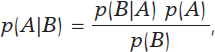
being p(A) the probability of event A, p(A|B) the associated probability A conditioned by the information that B occurred, and comparably p(B)> 0 and p(B|A). It is important to distinguish between probabilities p(A) and p(A|B). Both quantify the occurrence of A, but p(A) does so in absolute terms while p(B|A) does so in relative terms and conditioned by the information picked up in B. For example, nobody would question that the chances that a person may suffer from angina pectoris are higher if this person is hypertensive as opposed to not having that information available, p (Angina pectoris|Hypertension) > p (Angina pectoris).
Example I: Infections and tests
The prevalence that a certain infection affects any given population is .004. There is a test to detect its presence with a 94% sensitivity and a 97% specificity. We want to assess the chances that a person from such population is really infected if he tested positive for an infection.
We will use V and Vc to define a success that describes whether a person is infected or not, respectively. Therefore, p(V) = .004 and p(Vc) = .996. We’ll use (+) and (–) to describe a positive and negative test result for infection, respectively. In probabilistic terms, if a person is infected, he will test positive with a .94 probability, and negative with a .06 probability, p(+|V) = .94 and p(–|V) = .06 (false negative). If not infected, the person will test negative with a .97 probability and positive with a .03 probability, p(–|Vc) = .97 and p(+|Vc) = .03 (false positive).
According to Bayes’ theorem, the chances that a person is infected with a positive test result are
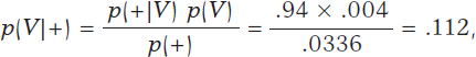
being p(+) = p(+|V) p(V) + p(+|Vc) p(Vc) = .0336 after implementing the total probability theorem (figure 1).
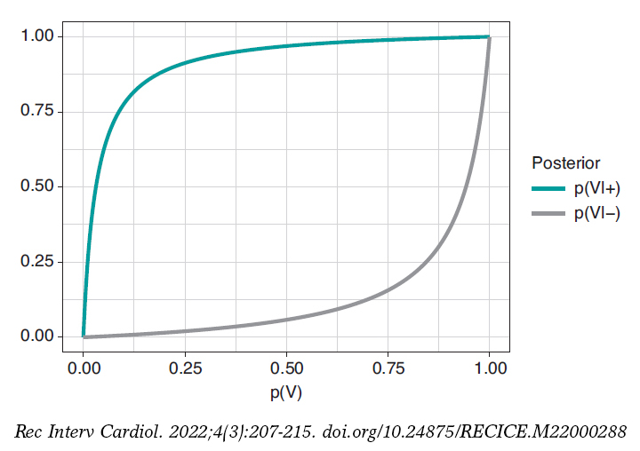
Figure 1. Posterior probability of infection with a positive test result p(V|+) (upper chart) and a negative test result p(V|–) (upper chart) in relation to the prior probability, p(V), of infection.
In principle, it is disconcerting that such a reliable test and with a positive test result for infection generates a small posterior probability, .112 favorable to the infection. However, if we take into consideration that the initial probability of being infected is p(V) = .004 and that, after the positive test result, probability is p(V|+) = .112, we’ll see that it has gone up from 4 to 112 by a thousand—has multiplied by a factor of 28—and we believe that the influence of the test result in such posterior probability is more relevant. Anyways, we would, at least, need a second test to increase the evidence for or against the infection.
Figure 2 shows 2 charts. The upper curve is the posterior probability of infection when the test is positive, p(V|+). The lower curve is the probability of infection too, but with a negative test result, p(V|–). In both cases, such posterior probabilities are represented in terms of prior probability, p(V), of being infected. When p(V) is close to 0, as it is the case with this example, the probability p(V|+) goes up a lot although, in absolute terms, it remains very low. On the contrary, when p(V) is close to 1, the probability p(V|–) will still be high despite evidence against a very reliable negative test result. The main element to understand this situation is that posterior probability, p(V|+) = .112, combines a very small probability of having an infection with a very high probability of testing positive when infected.
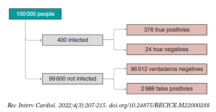
Figure 2. Approximate number of people infected, not infected, true positives, true negatives, false positives, and false negatives in a population of 100 000 inhabitants with an early prevalence for infection of .004 and a 94% sensitivity test and a 97% specificity test.
We’ll move on now to assess our results. The prevalence of infection, p(V) = .004 indicates that in a population of 100 000 people we should be expecting around 400 people infected and, approximately, 99 600 people not infected (figure 2). If the entire population were tested, we would expect to see that around 376 of the 400 people infected would test positive (true positives), as opposed to 24 (false negatives). In the group of healthy people, around 96 612 people would test negative (true negatives), but nearly 2988 people would test positive (false positives). If we looked at the number of people who tested positive, we’d have around 376 true positives, and 2988 false positives. Therefore, most people with a positive test (nearly 89%) would not actually be infected.
A second test with a positive result too would provide further evidence favorable to the infection. Its probability should be updated including the positive result of the second test as new information. If now (+1) and (+2) represent a positive test result for the first and second tests, the relevant probability would be p(V|+1,+2). The sequential use of Bayes’ theorem allows us to estimate such probability considering p(V|+1) = .112 as prior probability. The result obtained, p(V|+1,+2) = .798, is meaningful evidence favorable to an infection after 2 positive test results.
PARAMETER ESTIMATE
The true protagonists of basic Bayesian studies are probabilistic models governed by unknown parameters. These are at the core of Bayesian inferential machinery. We should mention that a parameter is a characteristic of a statistical population under study. Examples of parameters are the percentage of effectiveness of any given drug, the 5-year survival rate of soft tissue sarcoma, the basic reproduction factor R0 of an infection, etc. Parameters are estimated using partial information of the study population from data samples obtained through random procedures that guarantee their representativity and small population condition.
The most widely known probabilistic model is normal distribution with a dome-shaped symmetrical density function and defined by 2 different parameters, mean, µ, and standard deviation (σ). Mean is the center of gravity of distribution and corresponds to the peak of the dome. Standard deviation is a dispersion measurement that determines the width of the dome: in all normal distributions, the interval (µ − 3σ, µ + 3σ) includes 99.7% of the values of distribution. Therefore, the interval-related probability (−3, 3) in a normal distribution with mean = 0 and standard deviation = 1 would be the same as the one associated with the interval (−6, +6) of a normal distribution with mean = 0 and standard deviation = 2 (figure 3).
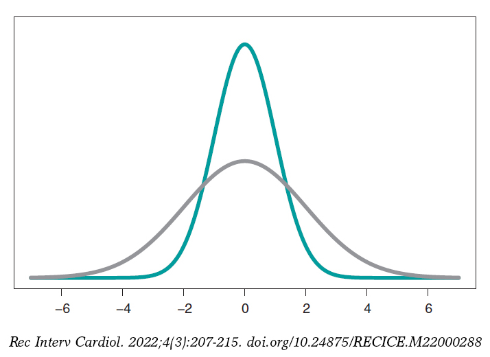
Figure 3. Chart of normal density with mean of 0, and standard deviation of 1 (green color), and normal density with mean of 0, and standard deviation of 2 (gray color).
Mean and standard deviation are unknown parameters in most studies based on normal data. In our case, and to avoid any technical complications, we’ll assume that the standard deviation is known. Therefore, the statistical process will only have eyes from the mean µ. Bayes’ theorem adapts itself to the territory of probability distributions with focus on the population mean symbol µ as parameter of interest according to the following formula
being p(μ) the previous distribution (or prior distribution) of μ that quantifies, in probabilistic terms, the initial information available on μ and p(μ | data), the posterior distribution of µ that contains the information on µ available when the initial information is added to data. The term p(data | μ) is the verisimilitude function of μ, a measurement that assesses the compatibility of data with the possible μ values. The element p(data) is the previous predictive distribution (also evidence in the automatic and machine learning setting), and assesses the plausibility of the data obtained.
Example II: the heart of boys and girls with spinal muscular atrophy
Falsaperla et al.6 present the results of an observational study on the heart electrical conduction system disorder that causes bradycardia or electrocardiographic abnormalities in boys and girls with spinal muscular atrophy type 1 and 2 (SMA1, and SMA2, respectively). We gained our inspiration from this study to build a simulated database. Therefore, the results from this example do not come from Falsaperla et al.6 and should not be compared to those from the original study.
We simulated the data on the PR interval length that extends from the origin of atrial depolarization until the origin of ventricular depolarization from 14 children with SMA2. We assumed a normal model with unknown measurement and known standard deviation. Out statistical goal was to estimate the mean.
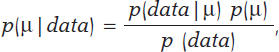
We’ll go on now with the Bayesian protocol. First, we need a previous distribution p(μ) to express our information of such parameter. Afterwards, we consider a scenario without new information on μ except for the information provided by data and use Jeffreys Prior to treat all possible μ values the same way.7 The posterior distribution of μ, p(μ | data), is a normal distribution with a mean of .13, and a standard deviation of .03/√∙14 seconds that we can graphically see on figure 4. We estimate that μ is .13 seconds, and directly assess the accuracy of such estimate through a credibility interval that tells us that the posterior probability of μ will be taking values between .114 and .146 seconds is .95. We give it a very low probability of .05 that μ will be > .146 or < .114.
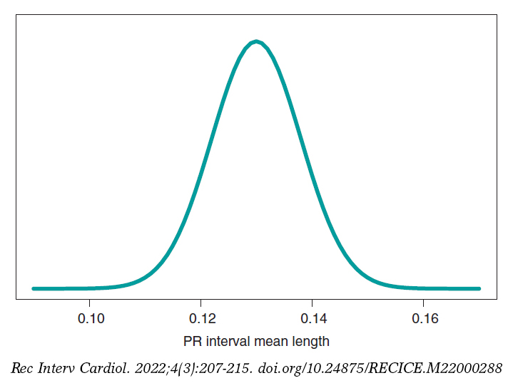
Figure 4. Posterior distribution of the PR interval mean length in children with spinal muscular atrophy type 2.
A frequentist analysis of this data would never allow direct probabilistic assessments of μ. A frequentist 95% confidence interval for μ would provide the same numerical results compared to the Bayesian interval. However, it should be interpreted in a completely different way. The frequentist 95% confidence interval is on the capacity of the interval to include μ true value, and not on the possible μ values. The interval built, (.114, .146), has a .95 probability of capturing μ true value, but also a .05 probability of not doing so. We should remember that the frequentist concept of probability prevents allocating probabilities to parameters and establishing direct probabilistic assessments of μ.
PREDICTING NEW OBSERVATIONS
Prediction and estimation are fundamental statistical concepts. We estimate parameters, but we predict data and experimental results always through distributions of probability.
The posterior predictive distribution of the results of a future experiment is built by combining the probabilistic model that correlates future data and parameters with posterior distribution. A significant aspect of predictive process regarding estimation is its greater uncertainty. Overall, the precision of estimations improves with larger samples, which means that in the hypothetical case of having all the data available, our estimation would be accurate. The process of prediction does not have such a feature. Although the precision of predictions increases parallel to the size of the sample, in the hypothetical case of having access to all the information from a population, error-free predictions would still be impossible.
Example II: the heart of boys and girls with muscular atrophy (continues)
In the estimation stage we studied the PR interval mean length in girls and boys with SMA2, learning based on a sample of 14 simulated data. Now we’ll be dealing with totally different situation. We have a kid with SMA2 who did not participate in the study. Our objective is to predict his PR interval length. The goal now is not to estimate population means with SMA2, but to predict the value of the PR interval length in a particular kid.
Figure 5 shows the posterior predictive distribution of the PR interval length of a new boy with SMA2. Although this prediction is based on information from 14 children from the sample, it is about a new boy with SMA2. The anticipated value of this new child’s PR interval length is .13 seconds. The accuracy of prediction is quantified through prediction intervals. In this case with a .95 probability, the anticipated value will be between .069 and .191 seconds.
Figure 5. Posterior predictive distribution of the PR interval length of a new child with spinal muscular atrophy type 2.
SIMULATION AND GROUP COMPARISON
The Bayesian protocol with the 3 basic elements, previous distribution, verisimilitude function, and posterior distribution is common to almost all kinds of settings, both the basic ones including some parameters, as well as the complex ones with many sources of uncertainty with complex hierarchical structures. It is a robust and easy-to-use protocol, and a powerful and appealing idea.
Difficulties appear if we want to extrapolate this protocol to real studies of certain complexity. It is in just a couple of these cases that an analytical expression for the posterior distribution of parameters can be achieved. Impossible, nonetheless, for posterior distributions associated with derived quantities of interest. In most studies, mathematics becomes complicated, and posterior distributions are difficult to obtain. In these cases, the MCMC methods come to the rescue of Bayesian analysis. They can simulate our estimates of the relevant posterior distribution and from them generate the inferences or predictions required by the study.
In the following example we’ll be showing the most basic situation we have discussed: starting with a target posterior (analytical) distribution we’ll be simulating posterior distributions of relevant, non-analytical quantities of interest.
Example III: acute myocardial infarction and stents
The following example has been inspired by Iglesias et al.8. This is a study of 1300 patients with acute myocardial infarction treated with percutaneous coronary intervention. Each patient was randomized to sirolimus-eluting stent implantation with degradable polymer (group S) or everolimus-eluting stent implantation with durable polymer (group E).
We compared both treatments in relation to the rate of deaths 12 months after treatment. A total of 35 out of the 649 patients from group S stopped treatment or were lost within first year of follow-up, and 24 died. In group E, initially with 651 patients, 25 were lost or stopped treatment, and 22 died. The presence of missing data due to losses to follow-up is an important issue that should be dealt with carefully. In this case we’ll omit it because our goal is to illustrate Bayesian procedures using the least possible technicalities.
We’ll start by analyzing the risk of death θs and θE in groups S and E, respectively 1 year into treatment. Since anybody from either one of the 2 groups can die, or not, within the first year of treatment, in each group, the probabilistic model is binomial distribution that will be describing the number of deaths reported. The risk of death from each group is a rate with values that range between 0 and 1. For each rate we’ll be selecting beta distribution because it’s the proper probabilistic model to use with rates and doesn’t pose any estimate difficulties. β distribution (that we’ll representi as Be(α, β)) has 2 different parameters, α > 0 and β > 0, that determine the way of the distribution as well as its mean and variance. It is a flexible distribution that can be symmetrical or asymmetrical, positive or negative (figure 6).
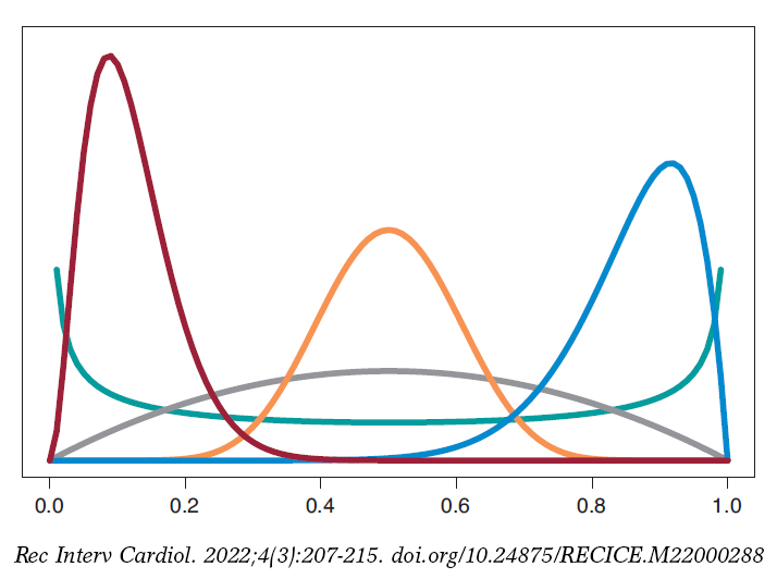
Figure 6. Chart of β densities: Be(.5, .5) in green color, Be(2, 2) in gray color, Be(3, 22) in maroon color, Be(12, 2) in blue color, and Be(12, 12) in pumpkin color.
The prior β distribution that best describes the lack of information is Be(.5, .5). Its justification only responds to theoretical criteria. In each group, the posterior distribution of the risk of death will also be β whose updated parameters can be obtained by adding the number of deaths and the number of people alive in the study to the 2 values 0.5 and 0.5 of the prior beta distribution:
p(θs) = Be(.5, .5); p(θs | data) = Be(24.5, 590.5),
p(θE) = Be(.5, .5); p(θE | data) = Be(22.5, 604.5).
The estimation of the risk of death in patients from groups S and E is the mean of its posterior distribution, .040 and .036, respectively. Also, with a .95 probability the risk of death of group S is between .026 and .057, and between .023 and .052 in group E. These results indicate that the rate of death from both groups is small, although slightly higher in group S. The 95% credibility interval—both of θs and θEis very informative (figure 7).
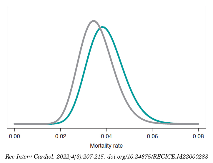
Figure 7. Posterior distribution of the mortality rate reported in patients from group S (green color) and group E (gray color).
We assume that our goal is to compare the 1-year mortality risk in both groups. Although the tool we could think of first is hypothesis testing (that we’ll introduce later on), the epidemiological and statistical literature on this regard is abundant, and 2 groups are often compared through relative risk (RR) or absolute risk (AR).9 The 1-year RR of mortality in patients with type S stents vs patients with type E stents is RR = θs/θE, a ratio between 2 rates. RR values < 1 are indicative that the mortality rate from group S is lower compared to group E while values > 1 are indicative of precisely the opposite. Since RR is defined through θs and θE, the information from both rates, expressed through its posterior distribution, can propagate to RR as a posterior probability distribution, p(RR | data) (figure 8). This distribution is not analytical, but it can come close to it through a Monte Carlo simulation from the 2 posterior distributions p(θs | data) and p(θE | data). Using this approximation, the posterior RR mean is 1.160, its standard deviation, .346, and the posterior probability of RR being >1 is .641. An analogue frequentist analysis would be more complicated from the mathematical standpoint and would not provide a direct probabilistic assessment of RR.
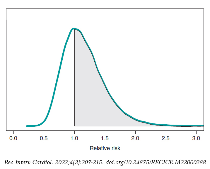
Figure 8. Posterior distribution of the relative risk of mortality at 1 year in patients with S-type stents vs patients with E-type stents. The shadow region is the probability, .641, that the mortality rate of group S is higher compared to group E.
If we compare both groups through the AR of mortality at 1 year, our goal would be AR = θs-θE. This is a difference between 2 rates that could take values between −1 and 1. Negative values will be indicative that the mortality rate of group E is higher compared to groups S while positive values will indicate just the opposite. figure 9 shows the AR posterior distribution.
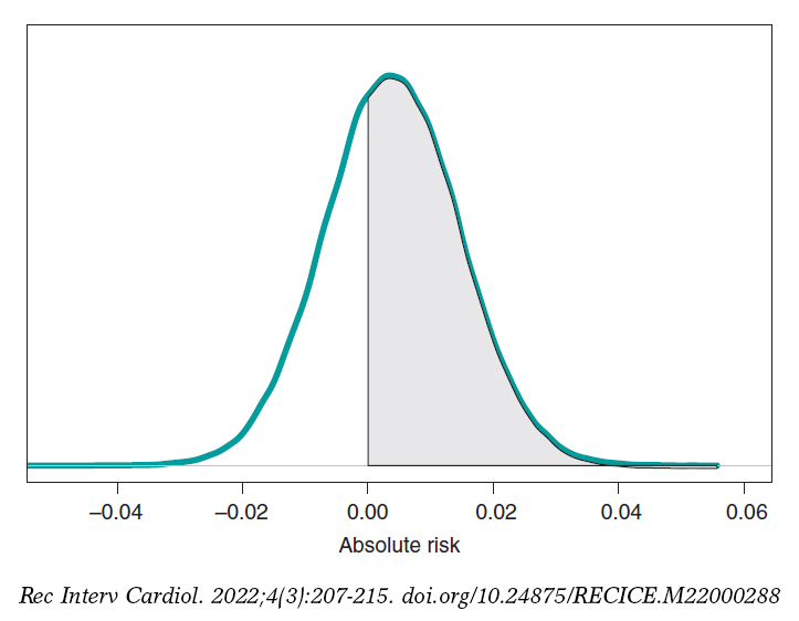
Figure 9. Posterior distribution of the absolute risk of mortality at 1 year in patients with S-type stents vs patients with E-type stents. The shadow region is the probability, .641, that the mortality rate of group S is higher compared to group E.
The posterior AR mean is .004, its standard deviation, .011, and with a .641 probability, the AR will be > 0.
HYPOTHESIS TESTING: FREQUENTIST P VALUES
Hypothesis testing is the topic that generates the most irreconcilable differences between the Bayesian and the frequentist scientific communities because it is here where the consequences of their different concepts of probability become more evident. Testing hypothesis means testing new theories. Most of the latest theories have a quiet appearance among the scientific community, but little by little they start accumulating evidence in their favor until the sitting evidence is debunked.
The most widely known and used concept in frequentist statistics is the P value, as well as its .05 value that in some studies appears as the magical number used to reject or accept hypotheses or scientific theories. P value is another tool in the frequentist inference armamentarium that simply does not exist in the Bayesian one regarding the testing of 2 different hypotheses: the null hypothesis H0 (that often represents the sitting scientific theory), and the alternative hypothesis H1 (the new theory). P values are always associated with data because without the latter there are no P values. Under these conditions, P value is the probability that a certain theoretical summary of data will be equal to the one observed or more incompatible with the null hypothesis supposing that such hypothesis holds true. Such compatibility is often represented by the P = .05 threshold. P values ≥ .05 keep confidence in the null hypothesis; P values < .05, however, are favorable to the alternative one.
The excessive, and sometimes, inappropriate use of P values in scientific studies is still under discussion in the statistical community. It started in small scientific circles, but the use of the P value soon became a somehow «magical» element rather than a scientific tool. Back in 2014, the American Statistical Association, one of the world’s leading statistical societies, approached this issue and drafted a document that has become the go-to guideline on this topic.10 The following ones are some of the conclusions on significant P values for the management of biometrical data:
- They are a probabilistic measurement of the compatibility of data with the null hypothesis. Smaller P values are associated with more data incompatibility with such hypothesis.
- Do not assess the probability that a hypothesis will hold true or not.
- The conclusions of a study should not only be based on whether a given P value exceeds this or that threshold. The use of the expression «statistically significant» (P < .05) to establish conclusions distorts all scientific procedures.
- Do not measure the size of an effect or the significance of a given result. All small effects can produce small P values when the size of the sample or the accuracy of measurements is big, and all big effects can generate big P values with small samples or imprecise observations.
The P value has been given an unfair treatment because it has been attributed fantastical and surreal properties that have turned against it. Controversy has shattered the scientific debate and encouraged criticism in scientific disciplines that use data to generate knowledge. The huge interest in today’s scientific reproducibility topics owes volumes to this debate.11-15
ACCUMULATING EVIDENCE FOR THE PROBABILISTIC ASSESSMENT OF NEW THEORIES
The Bayesian concept of probability is the key element to put hypotheses and theories to the test because it allows us to assign direct probabilities to both hypotheses and theories, both prior, p(theory holds true) and posterior, p(theory holds true|data ).16
Frequentist statistics is based on hypothesis testing using p-type probabilities (data|theory holds true) while Bayesian statistics is based on p-type probabilities (theory holds true|data). The p-type(data|theory holds true) frequentist probability assumes that the theory tested holds true, and based on that assumption assesses the concordance of data with such hypothesis. The p-type(theory holds true|data) Bayesian probability probabilistically assesses the certainty of the theory being tested in association with the data obtained.
The fundamental tool of Bayesian statistics to choose between hypotheses
H0: theory #1 holds true,
H1: theory #2 holds true,
based on a dataset is Bayes factor,17 the ratio between the probabilities associated with data according to both theories. It can also be expressed as the ratio between posterior odds (p(theory #1 holds true|data )/p(theory #2 holds true|data)) favorable to the certainty of theory #1 compared to theory #2 and the corresponding prior odds (p(theory #1 holds true)/p(theory #2 holds true). Like this:

Bayes factor (B) holds evidence favorable to the certainty of theory #1 (compared to theory #2) provided by data: it turns prior probabilities into posterior probabilities. In logarithmic scale, log (B), the Bayes factor is also known as «weight of evidence», a term coined by Turing back in Bletchley Park during Second World War. Small Bayes factor values give little support to H0 vs H1; however, big Bayes factor values provide extensive support to H0.
Example I: Infections and tests (continues)
Let’s go back to the data from example I: Vallivana needs to be diagnosed on an infection with 2 positive test results. This problem can be faced as 2 hypotheses being tested:
H0: Vallibana has an infection
H1: Vallibana doesn’t have an infection
We assume that Vallibana does not have any particular characteristics that give her a probability of infection different from the remainder of the population. Therefore, we know that p(Vallibana has an infection) = .004, and p(Vallibana doesn’t have an infection) = .996. Vallibana’s prior odds favorrable to the infection compared to non-infection are:

Vallibana takes the test, and it turns out positive (+1). She decides to retake it and tests positive again (+2.). Vallibana’s posterior odds favorable to the infection compared to non-infection are:

The Bayes factor in favor of Vallibana being infected, that is, the ratio between the posterior odds and the prior odds is 987.75. Indeed, this value provides strong evidence in favor of Vallibana being infected (+).
Example II: the heart of boys and girls with spinal muscular atrophy (continues)
Now let’s go back to the study conducted by Falsaperla et al.6 from example II that aimed to compare the PR interval mean length in girls and boys with SMA1 and SMA2—that we’ll refer to as μ1 and μ2, respectively—through hypothesis testing:
H0: μ2 ≤ μ1
H1: μ2 > μ1
where the null hypothesis, H0, claims that the PR interval mean length in girls and boys with SMA2 is shorter or equal to that reported in children with SMA1. The alternative hypothesis H1 says otherwise. Here we’ll be working with simulated normal data in both groups: n1 = 14 observations in the SMA1 group with sample mean and standard deviation values of .10 and .02 seconds, respectively, and n2 = 14 observations in the SMA2 group with sample mean and standard deviation values of.13 and .03 seconds, respectively.
What we´ll do is build an inferential process for the mean of each group separately. In both cases, we’ll be considering a neutral previous distribution that gives all prominence to data. figure 10 shows the posterior distribution of the mean of each group. Both distributions are rather separate from one another, which means that the posterior probabilities associated with each hypothesis will be very different as well: .002 for H0, and .998 for H1.
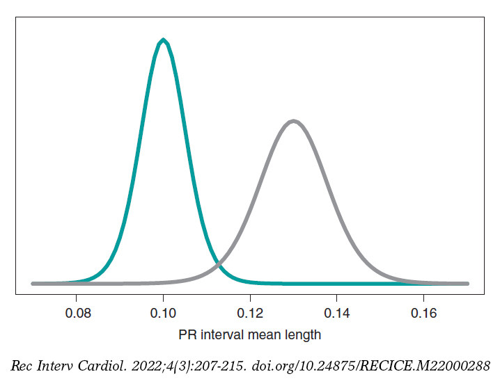
Figure 10. Posterior distribution of the PR interval mean length in girls and boys with spinal muscular atrophy type 1 (green color), and type 2 (gray color).
p(H0|data) = p(μ2 ≤ μ1|data) = .002
p(H1|data) = p(μ2 > μ1|data) = .998
On a roughly basis, it is 500 times more likely that H1 will hold true than not. In light of such an overwhelming piece of evidence the wise decision would be to choose H1. The frequentist treatment of this testing is based on the P value. In our case, we’d obtain a P value of .002, which would imply rejecting the null hypothesis in favor of the alternative one. Both methodologies propose the same decision and provide the same numerical results: probabilities of .002. However, both probabilities are conceptually different. Bayesian probability tests the null hypothesis based on the data reported. Frequentist probability assesses the data observed with the assumption that the null hypothesis will hold true.
Still following in the footsteps of Falsaperla et al.6 we wish to mention that our examples are not based on original cases. They are merely illustrative of Bayesian procedures. We’ll now be working with the P-wave on the electrocardiogram. We wish to compare the P-wave mean length in children with SMA1 and SMA2. We’ll be simulating 14 observations of the P-wave length in the group of children with SMA1 and compared it to children with SMAs. The sample mean and standard deviation is .09 and .05 seconds in group SMA1, respectively, and .07 and .03 seconds in group SMA2. We’ll be comparing the means of both groups through hypothesis testing:
H0: mean P-wave in SMA1 = mean P-wave in SMA2
H1: mean P-wave in SMA1 > mean P-wave in SMA2
based on Bayesian inferential process like the one from the previous example. figure 11 shows the posterior distribution of the P-wave mean length in both groups. There are fewer data from the group of girls and boys with SMA2 compared to the group with SMA1. The posterior probability associated with each hypothesis is:
p(H0 | data) = p(mean P-wave in SMA1 ≤ mean P-wave in SMA2 | data)
p(H1 | data) = p(mean P-wave in SMA1 > mean P-wave in SMA2 | data)
These results provide a significant piece of evidence favorable to the alternative hypothesis that is almost 8 times more likely than H0. From the frequentist standpoint, the P value associated with data would be .107 (>.05), which is why we would conclude that data does not provide enough evidence to reject H0. Bayesian decision could perfectly be the same. However, the Bayesian analysis provides a direct assessment on the certainty of both hypotheses. The findings from the Bayesian analysis could be used as previous information in future studies with more data. Therefore, the posterior distributions obtained (figure 11) would be prior distributions in this new study. Bayes’ theorem allows us to generate knowledge sequentially searching for evidence for or against different hypothesis.
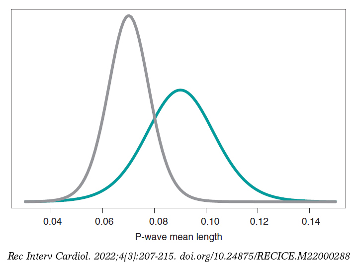
Figure 11. Posterior distribution of the P-wave mean length in girls and boys with spinal muscular atrophy type 1 (green color), and type 2 (gray color).
CARDIOLOGY POSES SOME OF DOUBTS ON THE IMPLEMENTATION OF METHODOLOGY IN CLINICAL TRIALS
One of the most controversial topics in Bayesian methodology is the selection of previous distributions. A Bayesian analysis will always allow us to avoid using any information on the amount of interest not provided by data. In this case, it works with previous distributions that play a neutral role in the learning process and that are useful only as the starting point of the Bayesian inferential protocol.
Previous informative distributions contain information that adds to the one provided by data like expert knowledge18-20 or results from previous studies.21,22 It is a highly valuable Bayesian characteristic in studies on which data is scarce like studies on rare diseases and orphan drugs. We should mention that inferential processes based on previous informative distributions should include sensitivity analyses of the results obtained regarding previously used distribution or distributions. Similarly, it has become popular to consider communities of previous distributions with diverse previous distributions—and a certain degree of skepticism or enthusiasm—with the effect under test because they provide a scientific framework of reference.
On many occasions, in clinical trials, the use of previous informative distributions reduces the sizes of frequentist samples based on preassigned values of the test power, and previous parameter estimates.22 An example of this situation is the BIOSTEMI trial.8 The 1300 patient-sample was estimated using Bayesian methods through a previous robust distribution as a mixture that included—in equal proportion—historical information of 407 patients from the BIOSCIENCE trial,23 and a practically non-informative distribution. The flexibility of Bayesian sequential learning is a key element of the so-called adaptative Bayesian designs24 that allow us to include additional information in different phases of the trial without damaging the consistency and reliability of results.
FUNDING
This study was partially funded by Biotronik Spain S. A, and by project PID2019-106341GB-I00 from the Spanish Ministry of Science and Innovation, and Universities of the Spanish Government.
AUTHORS’ CONTRIBUTIONS
C. Armero was involved in the structure, content, and drafting of this manuscript; P. Rodríguez, and J.M. de la Torre Hernández were actively involved in the review process of the manuscript final version.
CONFLICTS OF INTEREST
C. Armero, P. Rodríguez, and José M. de la Torre Hernández declared no conflicts of interest regarding the content, authorship, and publication of this manuscript. J.M. de la Torre Hernández is the editor-in-chief of REC: Interventional Cardiology. The journal’s editorial procedure to ensure impartial handling of the manuscript has been followed.
REFERENCES
1. Hawking S. A Brief History of Time: The Origin and Fate of the Universe. New York: Bantam; 1988.
2. McGrayne SB. La teoría que nunca murió: De cómo la regla de Bayes permitió descifrar el código Enigma, perseguir los submarinos rusos y emerger triunfante de dos siglos de controversia. Barcelona: Crítica; 2012.
3. Metropolis N, Rosenbluth A, Rosenbluth M, Teller A, Teller E. Equations of state calculations by fast computing machines. J Chem Phys. 1953;21:
1087-1092.
4. Robert CP, Casella G. A Short History of Markov Chain Monte Carlo: Subjective Recollections from Incomplete Data. Stat Sci. 2011;26:102-115.
5. Gelfand AE, Smith AFM. Sampling-based approaches to calculating marginal densities. J Am Stat Assoc. 1990;85:398-409.
6. Falsaperla R, Vitaliti G, Collotta AD, et al. Electrocardiographic Evaluation in Patients With Spinal Muscular Atrophy: A Case-Control Study. J Child Neurol. 2018;33:487-492.
7. Robert CP, Chopin N, Rousseau J. Harold Jeffreys’s Theory of Probability Revisited. Stat Sci. 2009;24:141-172.
8. Iglesias JF, Muller O, Heg D, et al. Biodegradable polymer sirolimus-eluting stents versus durable polymer everolimus-eluting stents in patients with ST-segment elevation myocardial infarction (BIOSTEMI): a single-blind, prospective, randomised superiority trial. Lancet. 2019;394:1243-1253.
9. Christensen R, Johnson W, Branscum A, Hanson TE. Bayesian Ideas and Data Analysis: An Introduction for Scientists and Statisticians. Boca Raton: CRC Press; 2011.
10. Wasserstein RL, Lazar NA. The ASA Statement on p-Values: Context, Process, and Purpose. Am Stat. 2016;70:129-133.
11. Goodman SN. Toward Evidence-Based Medical Statistics. 1: The P Value Fallacy. Ann Intern Med. 1999;130:995-1004.
12. Greenland S, Senn SJ, Rothman KJ, et al. Statistical tests, P values, confidence intervals, and power: a guide to misinterpretations. Eur J Epidemiol. 2016;31:337-350.
13. Halsey LG, Curran-Everett D, Vowler SL, Drummond GB. The fickle P value generates irreproducible results. Nat Methods. 2015;12:179-185.
14. Ioannidis JPA. Why Most Published Research Findings Are False. PLoS Med. 2005;2:e124.
15. Ioannidis JPA. The Proposal to Lower P Value Thresholds to .005. J Am Med Assoc. 2018;319:1429-1430.
16. Kruschke JK. Doing Bayesian data analysis: A Tutorial with R, JAGS, and Stan. 2nd ed. Amsterdam: Academic Press/Elsevier; 2015.
17. Kass RE, Raftery AE. Bayes Factors. J Am Stat Assoc. 1995;90:773-795.
18. Hampson LV, Whitehead J, Eleftheriou D, et al. Elicitation of Expert Prior Opinion: Application to the MYPAN Trial in Childhood Polyarteritis Nodosa. PLoS One. 2015;10:e0120981.
19. Mason AJ, Gomes M, Grieve R, Ulug P, Powell JT, Carpenter J. Development of a practical approach to expert elicitation for randomised controlled trials with missing health outcomes: Application to the IMPROVE trial. Clin Trials. 2017;14:357-367.
20. Jansen JO, Wang H, Holcomb JB, et al. Elicitation of prior probability distributions for a proposed Bayesian randomized clinical trial of whole blood for trauma resuscitation. Transfusion. 2020;60:498-506.
21. Grant RL. The uptake of Bayesian methods in biomedical meta-analyses: A scoping review (2005–2016). J Evidence-Based Med. 2019;12:69-75.
22. Spiegelhalter DJ, Abrams KR, Myles JP. Bayesian Approaches to Clinical Trials and Health-Care Evaluation. Chichester: Wiley; 2004.
23. Pilgrim T, Heg D, Roffi M, et al. Ultrathin strut biodegradable polymer sirolimus-eluting stent versus durable polymer everolimus-eluting stent for percutaneous coronary revascularisation (BIOSCIENCE): a randomised, single-blind, non- inferiority trial. Lancet. 2014;384:2111-2122.
24. Schmidli H, Gsteiger S, Roychoudhury A, O’Hagan A, Spiegelhalter D, Neuenschwander B. Robust meta-analytic-predictive priors in clinical trials with historical control information. Biometrics. 2014;70:1023-1032.
* Corrresponding author:
E-mail address: carmen.armero@uv.es (C. Armero).


